[CV] Performance Factors
CNN Performance Factors
It is very hard to have a fair comparison among different object detectors. There is no straight answer on which model is the best. For real-life applications, we make choices to balance accuracy and speed. Besides the detector types, we need to aware of other choices that impact the performance:1) Feature Extractors (VGG16, ResNet, Inception, MobileNet)
Feature extraction is a process of dimensionality reduction by which an initial set of raw data is reduced to more manageable groups for processing. Feature extraction is the name for methods that select and/or combine variables into features, effectively reducing the amount of data that must be processed, while still accurately and completely describing the original data set.A CNN is composed of two basic parts of feature extraction and classification. Feature extraction includes several convolution layers followed by max-pooling and an activation function. The classifier usually consists of fully connected layers.

2) Output strides for the extractor.
In CNN, stride controls how the filter convolves around the input volume. In other words, the amount by which the filter shifts. It is usually default set to 1.3) Input image resolutions
4) Matching strategy and IoU threshold (how predictions are excluded in calculating loss).
IoU = intersection over unionIntersection over Union is an evaluation metric used to measure the accuracy of an object detector on a particular dataset.
You’ll typically find Intersection over Union used to evaluate the performance of HOG + Linear SVM object detectors and Convolutional Neural Network detectors (R-CNN, Faster R-CNN, YOLO, etc.); however, keep in mind that the actual algorithm used to generate the predictions doesn’t matter. As long as we have these two sets of bounding boxes we can apply Intersection over Union.
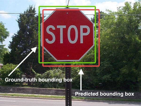
Below I have included a visual example of a ground-truth bounding box versus a predicted bounding box:

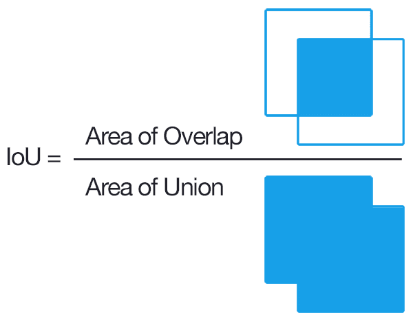
Computing Intersection over Union can therefore be determined via:

Examining this equation you can see that Intersection over Union is simply a ratio. In the numerator we compute the area of overlap between the predicted bounding box and the ground-truth bounding box. The denominator is the area of union, or more simply, the area encompassed by both the predicted bounding box and the ground-truth bounding box.
5) Non-max suppression IoU threshold.
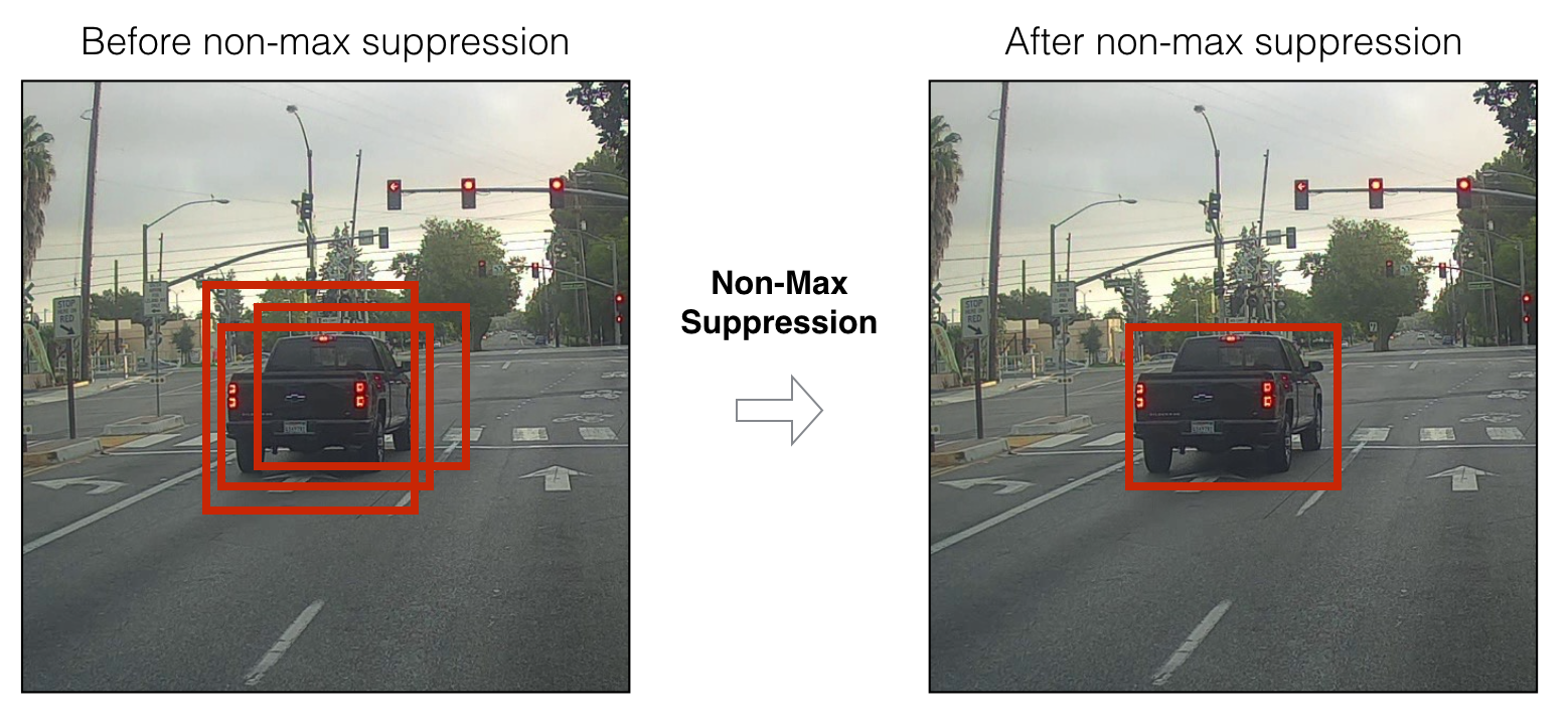
Typical Object detection pipeline has one component for generating proposals for classification. Proposals are nothing but the candidate regions for the object of interest. Most of the approaches employ a sliding window over the feature map and assigns foreground/background scores depending on the features computed in that window. The neighbourhood windows have similar scores to some extent and are considered as candidate regions. This leads to hundreds of proposals. As the proposal generation method should have high recall, we keep loose constraints in this stage. However processing these many proposals all through the classification network is cumbersome. This leads to a technique which filters the proposals based on some criteria ( which we will see soon) called Non-maximum Suppression.Input: A list of Proposal boxes B, corresponding confidence scores S and overlap threshold N.
Output: A list of filtered proposals D.
Algorithm:
- Select the proposal with highest confidence score, remove it from B and add it to the final proposal list D. (Initially D is empty).
- Now compare this proposal with all the proposals — calculate the IOU (Intersection over Union) of this proposal with every other proposal. If the IOU is greater than the threshold N, remove that proposal from B.
- Repeat step 1 and 2 until there are no more proposals left in B.
Now if you observe the algorithm above, the whole filtering process depends on single threshold value. So selection of threshold value is key for performance of the model. However setting this threshold is tricky. Let us see this scenario. Assume that the overlap threshold N is 0.5. If there is a proposal with 0.51 IOU and has good confidence score, the box will be removed even though the confidence is higher than many other boxes with less IOU. Because of this, if there are two objects side by side, one of them would be eliminated. A proposal with 0.49 IOU is still kept even though its confidence is very low. Of course this is the known issue with any threshold based technique. Now how do we deal with this? You can read about Soft-NMS.
6) Hard example mining ratio (positive v.s. negative anchor ratio).
Anchor boxes are a set of predefined bounding boxes of a certain height and width. These boxes are defined to capture the scale and aspect ratio of specific object classes you want to detect and are typically chosen based on object sizes in your training datasets. During detection, the predefined anchor boxes are tiled across the image. The network predicts the probability and other attributes, such as background, intersection over union (IoU) and offsets for every tiled anchor box. The predictions are used to refine each individual anchor box. You can define several anchor boxes, each for a different object size.The network does not directly predict bounding boxes, but rather predicts the probabilities and refinements that correspond to the tiled anchor boxes. The network returns a unique set of predictions for every anchor box defined. The final feature map represents object detections for each class. The use of anchor boxes enables a network to detect multiple objects, objects of different scales, and overlapping objects.
When using anchor boxes, you can evaluate all object predictions at once. Anchor boxes eliminate the need to scan an image with a sliding window that computes a separate prediction at every potential position. Examples of detectors that use a sliding window are those that are based on aggregate channel features (ACF) or histogram of gradients (HOG) features. An object detector that uses anchor boxes can process an entire image at once, making real-time object detection systems possible.
YOLO for instance, uses NMS after generating lots of detection candidates in the image.

TODO: http://www.erogol.com/online-hard-example-mining-pytorch/
7) The number of proposals or predictions.
8) Boundary Box Encoding
9) Data Augmentation
Having a large dataset is crucial for the performance of the deep learning model. However, we can improve the performance of the model by augmenting the data we already have. Deep learning frameworks usually have built-in data augmentation utilities, but those can be inefficient or lacking some required functionality.Data augmentation is a strategy that enables practitioners to significantly increase the diversity of data available for training models, without actually collecting new data. Data augmentation techniques such as cropping, padding, and horizontal flipping are commonly used to train large neural networks. However, most approaches used in training neural networks only use basic types of augmentation. While neural network architectures have been investigated in depth, less focus has been put into discovering strong types of data augmentation and data augmentation policies that capture data invariances.
A list of image augment tools are here: https://towardsdatascience.com/data-augmentation-for-deep-learning-4fe21d1a4eb9
10) Training Dataset
11) Use of multi-scale images in training or testing (with cropping)
12) Which feature map layer(s) for object detection
A feature map, or activation map, is the output activations for a given filter (a1 in your case) and the definition is the same regardless of what layer you are on.Feature map and activation map mean exactly the same thing. It is called an activation map because it is a mapping that corresponds to the activation of different parts of the image, and also a feature map because it is also a mapping of where a certain kind of feature is found in the image. A high activation means a certain feature was found.
A "rectified feature map" is just a feature map that was created using Relu. You could possibly see the term "feature map" used for the result of the dot products (z1) because this is also really a map of where certain features are in the image, but that is not common to see.
13) Localization Loss Function
Broadly, loss functions can be classified into two major categories depending upon the type of learning task we are dealing with — Regression losses and Classification losses.In classification, we are trying to predict output from set of finite categorical values i.e Given large data set of images of hand written digits, categorizing them into one of 0–9 digits.
Regression, on the other hand, deals with predicting a continuous value for example given floor area, number of rooms, size of rooms, predict the price of room.
A) Regression Loss
Ai) Mean Square Error (MSE)/Quadratic Loss/L2 Loss
However, due to squaring, predictions which are far away from actual values are penalized heavily in comparison to less deviated predictions. Plus, MSE has nice mathematical properties which makes it easier to calculate gradients.
Aii) Mean Absolute Error/L1 Loss

This measures the magnitude of error without considering their direction. Unlike MSE, MAE needs more complicated tools such as linear programming to compute the gradients. Plus MAE is sensitive to outliers since it does not make use of square.
Aiii) Mean Squared Logarithmic Error (MSLE)

Use MSLE when doing regression, believing that your target, conditioned on the input, is normally distributed, and you don’t want large errors to be significantly more penalized than small ones, in those cases where the range of the target value is large.
Example: You want to predict future house prices, and your dataset includes homes that are orders of magnitude different in price. The price is a continuous value, and therefore, we want to do regression. MSLE can here be used as the loss function.
B) Classification Loss
Bi) Hinge Loss/Multi class SVM Loss
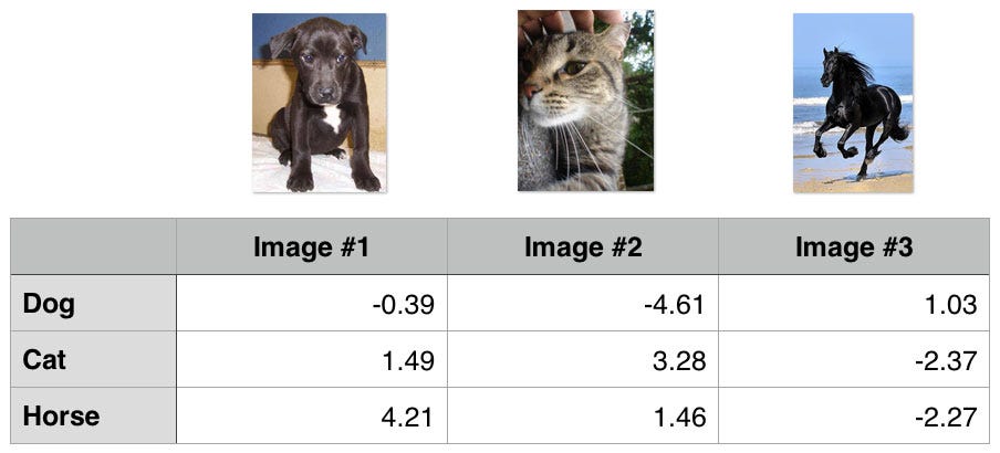
In simple terms, the score of correct category should be greater than sum of scores of all incorrect categories by some safety margin (usually one). And hence hinge loss is used for maximum-margin classification, most notably for support vector machines. Although not differentiable, it’s a convex function which makes it easy to work with usual convex optimizers used in machine learning domain.

## 1st training example
max(0, (1.49) - (-0.39) + 1) + max(0, (4.21) - (-0.39) + 1)
max(0, 2.88) + max(0, 5.6)
2.88 + 5.6
8.48 (High loss as very wrong prediction)
Bii) Cross Entropy Loss/Negative Log Likelihood
This is the most common setting for classification problems. Cross-entropy loss increases as the predicted probability diverges from the actual label.
Biii) Categorial Cross Entropy
Categorical cross entropy is a loss function that is used for single label categorization. This is when only one category is applicable for each data point. In other words, an example can belong to one class only.
Use categorical crossentropy in classification problems where only one result can be correct.
Example: In the MNIST problem where you have images of the numbers 0,1, 2, 3, 4, 5, 6, 7, 8, and 9. Categorical crossentropy gives the probability that an image of a number is, for example, a 4 or a 9.

14) Deep Learning Software platform used.
15) Training and Configurations including batch size, input image resize, learning rate and learning rate decay.
Resources:
https://deepai.org/machine-learning-glossary-and-terms/feature-extractionhttps://adeshpande3.github.io/A-Beginner%27s-Guide-To-Understanding-Convolutional-Neural-Networks-Part-2/
https://www.pyimagesearch.com/2016/11/07/intersection-over-union-iou-for-object-detection/
https://www.quora.com/How-does-non-maximum-suppression-work-in-object-detection
https://www.mathworks.com/help/vision/ug/anchor-boxes-for-object-detection.html
http://www.erogol.com/online-hard-example-mining-pytorch/
https://stats.stackexchange.com/questions/291820/what-is-the-definition-of-a-feature-map-aka-activation-map-in-a-convolutio
https://towardsdatascience.com/common-loss-functions-in-machine-learning-46af0ffc4d23
https://peltarion.com/knowledge-center/documentation/modeling-view/build-an-ai-model/loss-functions/categorical-crossentropy
https://leonardoaraujosantos.gitbooks.io/artificial-inteligence/content/object_localization_and_detection.html
https://lilianweng.github.io/lil-log/2018/12/27/object-detection-part-4.html#loss-function


Comments
Post a Comment